IceCube Dust Map
Accounting for the distortions and fine structure in dust will improve the detector model. Laser Dust Logger profiles correspond closely to dust measurements in Antarctic ice cores. Images taken in IceCube boreholes 21, 50, 66, 52, 10, 2, 86 and 14 between 2004 and 2011 (Fig. 1) show highly detailed, repeatable structure. By aligning dust features in depth we can combine all optical logs to form an "average" dust profile. Features have been mapped automatically using Dynamic Time Warping (described here) at full ~2 mm effective resolution. In some instances, small mapping errors may wash out fine scale features (<<1 m) in forming the composite. This composite South Pole optical profile is one of the best resolved and most stratigraphically coherent record of Antarctic dust of the last glacial period (Fig. 2).

 Fig 2. (Left) Averaged South Pole laser Dust Logger profile (unpublished) linearly scaled to measurements of insoluble dust in the ice core at Dronning Maud Land. The optical composite is the best resolved Antarctic dust record available. (Right) Dust Logger composite compared with Dome C core calcium from continuous flow analysis [Lambert et al. 2012].
To determine dust profiles for other strings we can interpolate or extrapolate using the eight dust logs as reference points. Positions within the convex hull defined by the logs can be interpolated with a standard natural neighbor method (Delaunay tessellation). External locations must be extrapolated and we use a modified ridge estimator. Extrapolated dust profiles for strings not enclosed by dust logs, e.g. 75-78, should be treated with caution. Note that Hole 21 was only logged to 2113 m, so the bottom ~350 meters in the southeast corner must also be extrapolated.
Fig 2. (Left) Averaged South Pole laser Dust Logger profile (unpublished) linearly scaled to measurements of insoluble dust in the ice core at Dronning Maud Land. The optical composite is the best resolved Antarctic dust record available. (Right) Dust Logger composite compared with Dome C core calcium from continuous flow analysis [Lambert et al. 2012].
To determine dust profiles for other strings we can interpolate or extrapolate using the eight dust logs as reference points. Positions within the convex hull defined by the logs can be interpolated with a standard natural neighbor method (Delaunay tessellation). External locations must be extrapolated and we use a modified ridge estimator. Extrapolated dust profiles for strings not enclosed by dust logs, e.g. 75-78, should be treated with caution. Note that Hole 21 was only logged to 2113 m, so the bottom ~350 meters in the southeast corner must also be extrapolated.

 Fig 3. (Left) Dust feature depth maps for all holes relative to Hole 86; the seven basis maps are in red. (Right) Hole 86, logged in 2009-10, is closest to the origin of the array coordinate system. The Hole 66 log reached the farthest back in time.

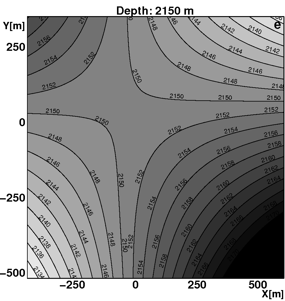
 Fig 4. (Left, a) Downhill gradients in dust layers across IceCube modeled using modified ridge estimation. (Right) Movie of dust isochrons changing with depth.
(Below, b-f) Dust isochron at selected depths; each contour line indicates a 2 m change in elevation.


Detector variables are useful for evaluating the map, particularly at locations far from dust log reference points. Fig. 6 shows stacked track miss probability for strings with few if any bad DOMs (provided by Dawn Williams) and which are close to dust logged holes, overlaid with average dust and all warped to the depths of dust features for String 86 (near the array center). Fine details in dust structure become more consequential in cleaner ice. Features which appear as spikes in the dust logger signal can strongly affect the detector response but are currently not accounted for in simulations. Although relatively thin layers, these pronounced local maxima in scattering and absorption tend to dump photons.

 Fig 5. (Left) Stacked track miss probability (based on 200 m track detection probability) overlaid with average dust. Spike-like features resulting from layers of volcanic or locally strong dust fallout can strongly affect the detector response, but are not currently modeled. (Right) Stacked, inverted software LC rate overlaid with average dust.
The Map
 Fig 6. Dust layers mapped with an algorithm are stacked to form a composite average dust profile.
Individual composite dust profile for any string, approximately normalized to Dome C core concentration (mass ppb).
Fig 6. Dust layers mapped with an algorithm are stacked to form a composite average dust profile.
Individual composite dust profile for any string, approximately normalized to Dome C core concentration (mass ppb).
<Depth> <Dust_Concentration>
A tarball of all 86 profiles can be downloaded here.
Version Aug. 15, 2011
Individual spline-smoothed dust feature maps relative to Hole 86. <Depth> <Depth - Depth86>
A tarball of all 85 maps can be downloaded here.
South Pole age vs. depth
We continue to refine the South Pole age scale, now nearly 90% of the way to bedrock. At shallow and intermediate depths in bubbly ice, we used ash and dust layers from Dust Logger images that we could unambiguously associate with layers we detected in logs at Siple Dome and Dome C. In the deep clear ice we tied our logs to dust measurements in the Dome C and EDML ice cores. In Figure 7 we have extrapolated to bedrock using 1) a simple two-parameter quadratic depth transformation (0.389d - 0.56x10⁻³d2) of Dome C age, forced through the origin and matched to our deepest dust features, and 2) a polynomial fit to all control points, including one below 2500 m extrapolated from Titan Dome Base, taken to be 165 kyr at 2850 m.
Preliminary South Pole age versus depth (EDC3) for Hole 86. <Depth86> <Age (kyr B.P.)>
 Fig 7. South Pole age versus depth for Hole 86 (unpublished) on the EDC3 timescale. The dashed red curve is a polynomial fit through our volcanic tie points, dust tie points, and a bedrock age estimate extrapolated from Titan Dome; the solid blue curve is Dome C age versus depth scaled to match SP tie points; the dotted gray curve was the prediction based on early AMANDA observations and a simple model. An increase in accumulation rate during the Eemian period is evident in the Dome C analog.
Ash Layers
From these images and dust logs made at Siple Dome (West Antarctica) and Dome C (East Antarctica), together with ice core measurements, we can identify certain depositions at South Pole to be volcanic. We currently have around 20 candidate ash layers, with roughly half lying at IceCube instrumented depths.


 Fig 8. Volcanic ash layers in the ice at South Pole present optical singularities that can appear light or dark, depending on ash albedo and context. Only the first has been confirmed in a shallow ice core; a few others can be associated with layers at other locations which have been chemically confirmed as volcanic.
How the Dust Logger works
The Dust Logger makes high definition images of optical effects due to particulates and bubbles, integrated over an area of order m2 of the horizon. Residual air bubbles reduce the contrast of dust scattering and make unambiguous identification of horizons increasingly difficult shallower than about 1200 m and into the Last Glacial Maximum around ~1150 m. In all dust profiles the effects of bubble scattering have been removed with an amplitude correction of 0.37% per meter above 1350 m (Fig. 9). At depths below 1350 m where all bubbles have converted to air hydrates, the logger signal closely tracks insoluble mineral dust (Fig. 2).
 Fig 9. An ad hoc amplitude correction, to remove the effects of bubble scattering above 1350 m, has been applied to all Dust Logger profiles.
The logger uses a computer-controlled 404 nm laser line generator, digital photon counter for light detection and a precision Paroscientific pressure sensor for primary depth determination. Annular black nylon brushes function as baffles to intercept stray photons and sweep detritus, particularly ice crystals, from the light path. To log Holes 21 and 50 we permanently affixed the probe to the detector string and acquired data while the string was deployed; during the first log in Hole 21, telemetry with the probe was lost below 2113 meters. In the four subsequent boreholes we used the Robertson logging winch to deploy a ruggedized instrument which we could hoist back to the surface, making profiles on both the down and up trips and recovering the device. Data are sent as 10-ms samples to the surface using DSL communication. Logging depth is reconstructed from both pressure readings and winch payout, surveys of the snow surface, well distance to the top of the water column and corrections for water compressibility and cable stretch. Absolute logger depth accuracy is probably limited to a meter or two, while relative uncertainty over moderate depth intervals is negligible.
References:
- EPICA community members, Eight glacial cycles from an Antarctic ice core, Nature 429, 623-628 (2004).
- F. Parrenin et al., The EDC3 chronology for the EPICA Dome C ice core, Clim. Past 3, 485-497 (2007).
- P.Buford Price and The AMANDA Collaboration, On the age vs depth and optical clarity of deep ice at the South Pole, J. Glaciol. 41, 445-454 (1995).
- Urs Ruth, pers. comm.
- Matthias Bigler, pers. comm.
- Regine Röthlisberger et al., Dust and sea-salt variability in central East Antarctica (Dome C) over the last 45 kyrs and its implications for southern high-latitude climate, GRL 29, 1963 (2002).
- Martin J. Siegert and R. Hodgkins, A stratigraphic link across 1100 km of the Antarctic ice sheet between the Vostok ice core site and Titan Dome (near South Pole), Geophys. Res. Lett. 27, 2133-2136 (2000).

